Carleton University · Capstone project · 2011–2012
I supervised MuscleMate, a wearable interface that turned forearm muscle activity into computer input. Nick Stupich, Mark Klibanov, Musabbir Khan, and Amrita Sandhu built the acquisition electronics, embedded signal processing, recognition software, and applications as one working system.
A contraction could advance a presentation, continuously control a helicopter in a game, or form part of a recognizable gesture. The project brought a useful question into focus: which representation of a muscle signal makes the intended action easiest to distinguish?
My key contribution to that question was the natural-log transformation of the EMG frequency features. It exposed the separation between activation levels and made the geometry of a separating hyperplane clear. That insight also led to a practical way of estimating continuous muscle activation.
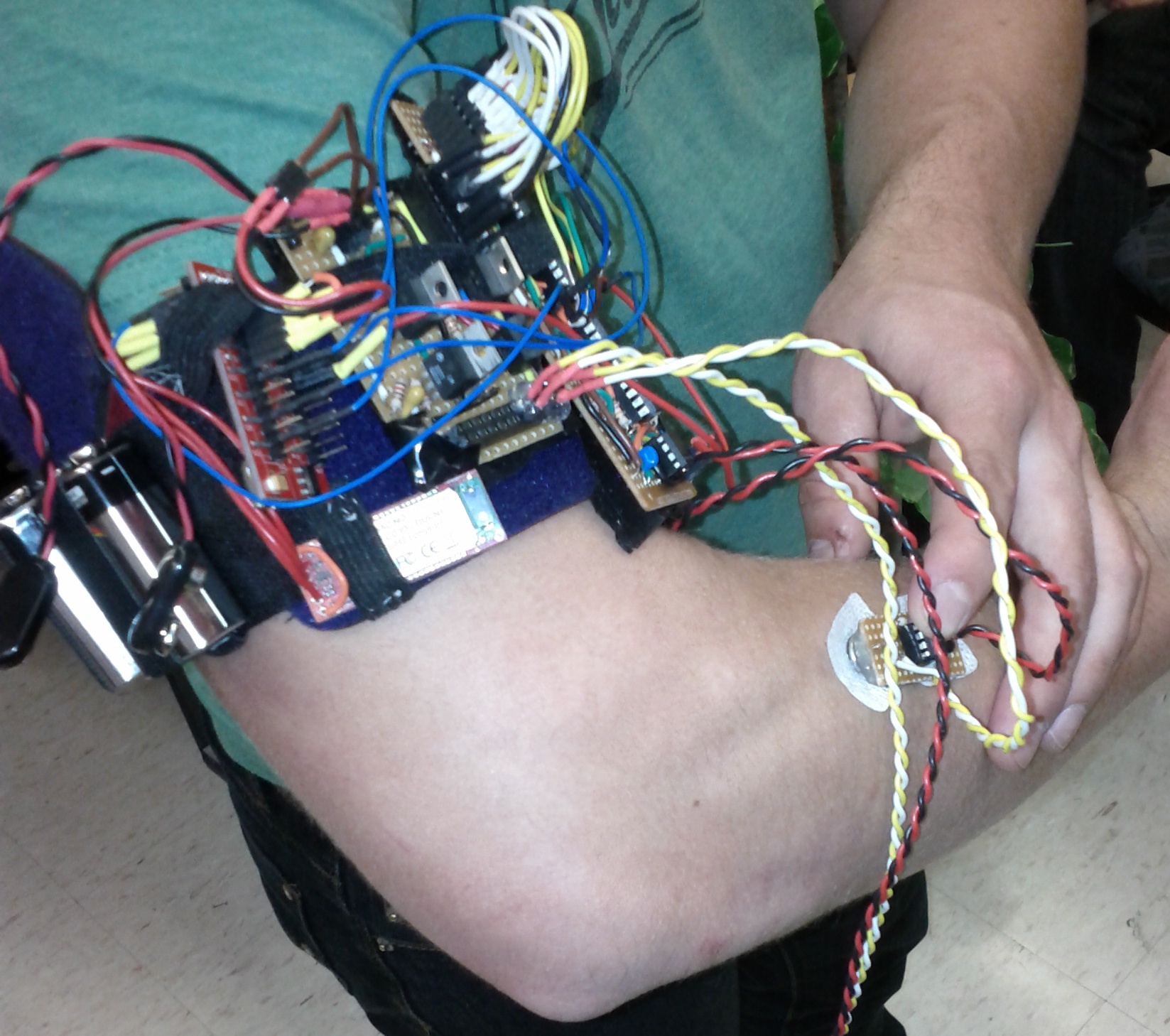
- Acquisition
- 3 channels
- Sampling
- 1,024 Hz
- FFT window
- 256 samples
- Representation
- 8 bins / channel
Building the wearable electronics
The electronics had to preserve a small differential signal while the user moved. Each sensor placed an AD620 instrumentation amplifier close to the electrode pair. Short connections brought the signal into the amplifier; subsequent stages selected the frequency band, controlled gain, and translated the waveform into the microcontroller’s input range.
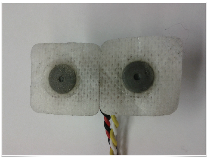
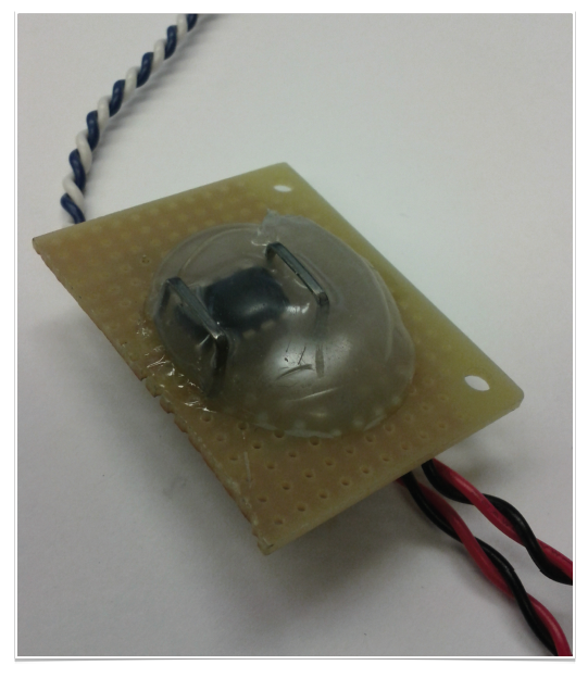
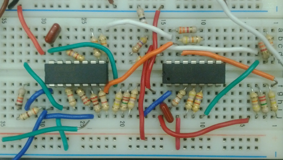
Several filter implementations were built and measured. Continuous-time UAF42 circuits provided an initial platform for studying passband and notch responses. The final conditioning design used a MAX7480 low-pass filter and an MF10 dual switched-capacitor filter for the 60 Hz and 120 Hz notches. Clock tuning placed those notches on the interference frequencies; the measured settings were 5,976 Hz and 11,952 Hz for the two MF10 sections.
Gain control linked the analog circuit to the firmware. A pulse-width-modulated output, smoothed into a control voltage, adjusted a JFET resistance in the amplifier feedback path. The firmware tracked mean-square deviation about ADC midscale and selected the gain for each channel. It also retained the gain setting when scaling the acquired samples, keeping changes in electronic gain associated with the signal values used for analysis.
Designing around a 10-bit converter
The ADC accepted a 0–3.3 V signal. Clipping and a DC-offset stage placed the conditioned waveform around 1.65 V. Automatic gain control helped use that input range across changes in contraction strength and electrode contact.
Separate channel boards, a regulated supply powered by two 9 V batteries, and a fabric strap made the complete instrument portable. This modular construction let the students test each stage and then assemble the full signal path.
From samples to frequency features
The Fez Mini microcontroller converted each signal into a compact frequency representation before sending it over Bluetooth. A 256-sample window at 1,024 samples per second spans 250 ms and gives 4 Hz frequency spacing. Successive overlapping windows allowed the software to update its interpretation as a contraction developed.
1,024 samples/s
4 Hz spacing
8 frequency bins
PC or Android
Δf = fs/N = 4 Hz
The real-input FFT used the symmetry of the spectrum to reduce memory and computation. Twenty-four magnitudes were grouped into eight features per channel. The retained frequencies stepped around the 60 Hz interference component:
Timing and memory were active design constraints. The native routines shared a 10,236-byte code-and-data region. Timer interrupts gave sampling priority while FFT and transmission work ran between acquisitions. A real-input transform, compact trigonometric tables, and a custom packet format kept the processing small enough for the platform.
The wireless protocol carried one scale value and eight feature values per channel, with a reserved delimiter for packet alignment. Channel-selection commands let the host choose which sensors to acquire. This separated the time-critical acquisition work from the training and application logic.
The logarithmic insight
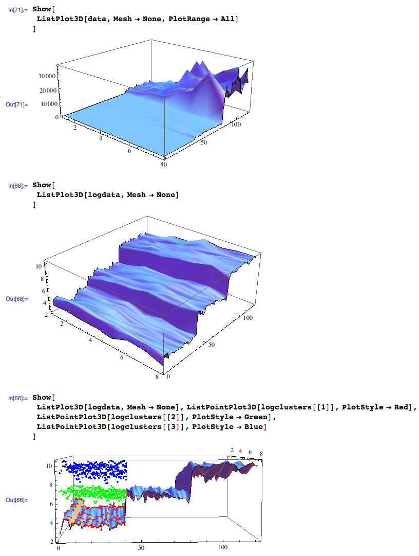
We recorded the forearm extensors at three instructed effort levels: relaxed, intermediate, and maximum perceived contraction. On the original feature scale, the largest values dominated the display. I took the natural logarithm of the data in Mathematica and shared the result with the students. The transformed surface revealed three distinct regions.
The important change was geometric. For a positive frequency-bin magnitude pi, define the transformed feature
A multiplicative change becomes an additive displacement: ln(a p) = ln(a) + ln(p). Large amplitude ratios become manageable distances, and the intermediate activation level becomes easier to distinguish. This gave us a useful coordinate system for both separation and interpolation.
In these coordinates, a linear decision boundary has the form wTz + b = 0. Written in the original magnitudes, the same boundary is a weighted product:
∏i piwᵢ = e−b
A simple hyperplane can therefore express a structured relationship among the original EMG features. Choosing the representation changes what a linear model can describe.
From features to muscle control
The software exposed two complementary outputs from each acquisition window: a discrete muscle-state decision and a continuous activation estimate. Each model was trained for the user and the action being controlled.
A separating hyperplane for muscle state
The students implemented a linear support vector machine using LIBSVM. Training paired frequency-bin vectors with labels captured from a key press or a touch input. Each output received its own model. At runtime, the decision reduced to a weighted sum and threshold:
ŷ = sign(s(x))
The weights determine the orientation of the separating hyperplane and the contribution of each frequency bin. In the tested linear SVM, x contained the acquired frequency features; the logarithmic transformation above supplied an additional coordinate system for studying separation. The trained weight vector also offered a way to inspect which parts of the spectrum carried the muscle-state information.
For the recorded binary muscle-state data, ten-fold cross-validation gave approximately 99% accuracy for the linear SVM, compared with approximately 96% for a threshold on summed features. The SVM used a cost parameter of 0.001. Errors concentrated around changes of state, connecting classifier performance to the 250 ms observation window and the timing of the training labels.
A log-domain estimate of activation
The continuous output used the logarithmic features directly. For each bin, the students fitted a line from log magnitude to the instructed effort level. They combined the individual estimates using their Pearson correlations with the training target:
â = (∑i ρiai) / (∑i |ρi|)
Here mi and ci are the fitted slope and intercept, and ρi measures the association between a bin and the target. Bins that tracked the instructed effort contributed more strongly. The output was a user-calibrated control level, which the helicopter game turned into vertical acceleration.
Recognizing a gesture through time
A gesture is a sequence. Two performances can share the same order of muscle events while differing in duration. The students used dynamic time warping (DTW) to align feature sequences and compare their shapes across changes in execution speed.
Let ui be a feature vector from the incoming sequence and vj one from a stored example. The local cost is their Euclidean distance. The accumulated cost follows
+ min{D(i−1,j),
D(i,j−1), D(i−1,j−1)}
A diagonal step advances both sequences. A horizontal or vertical step allows one sequence to advance while the other holds its position. The resulting alignment accommodates local stretching and compression of the gesture.
The implemented recognizer compared 0.6-second sequences with stored examples. Training estimated a distance threshold from matches to the same gesture and matches to other activity. A penalized subsequence variant allowed the alignment to start or end within a recording, with a cost for the fraction omitted. This made the treatment of uncertain gesture boundaries part of the recognition method.
| Method | Gesture distance mean ± SD | Other activity mean ± SD | Separation |
|---|---|---|---|
| Basic DTW | 1,403 ± 294 | 4,743 ± 2,206 | 1.3 |
| Penalized subsequence | 578 ± 34 | 1,554 ± 667 | 1.4 |
Separation is the difference between the two means divided by the sum of their standard deviations. Both methods separated the recorded classes; the penalized subsequence method gave a modest increase in this measure. The experiment established a sequence-matching approach alongside the real-time muscle-state and activation outputs.
Putting muscle control to work
The PC and Android software shared a useful division of responsibility. A backend received and decoded the Bluetooth stream, collected labelled training examples, built models, and delivered predictions. Applications used those outputs to define an interaction.
Helicopter game
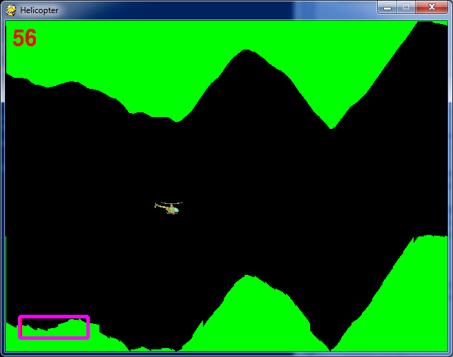
The player trained at three effort levels, then controlled ascent and descent by contracting and relaxing a chosen muscle. An on-screen power meter exposed the estimated activation. The narrowing cave made response timing and smooth control tangible.
Android interfaces
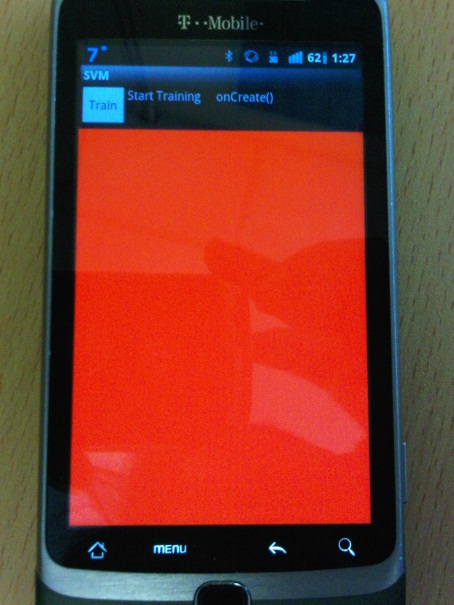
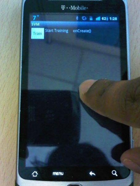
Colour Changer and Tone Generator connected muscle-state predictions to screen colour and sound. Touch input supplied training labels. Bluetooth acquisition and model computation ran alongside the interface, with synchronization managing the transition from training to prediction.
Presentation control
Binary muscle outputs mapped to forward and backward slide commands. A one-second interval between changes converted sustained activation into deliberate navigation. This exposed an application-level design question: the cost of an unintended slide change differs from the cost of waiting slightly longer for a deliberate command.
Related work in myoelectric interfaces places these continuous-control and gesture-command applications in their broader technical context.
From capstone to wearable research
The capstone joined an end-to-end acquisition instrument with trainable software and working applications. Students could follow a change in electrode contact through the analog circuit, inspect its effect in the frequency features, and observe the resulting application response. That connection between the physical signal and the user’s action became central to my subsequent wearable research.
The team received the Department of Electronics awards for best oral presentation and best poster, then first place in the Carleton Student IEEE and IEEE Eastern Ontario paper competitions. First place in the Faculty capstone competition brought $40,000 for continued development.
We subsequently expanded from three to eight channels and developed an armband with removable electrodes. Dedicated hardware used an ADS1298 eight-channel, 24-bit acquisition device, AD8222 instrumentation amplifiers, an LPC1343 processor, Bluetooth, and battery/USB power management. The work grew into textile-integrated muscle sensing, electrode calibration, and combined muscle and motion analysis.